Risk, Return, and Cost of Capital
Created by David Moore, PhD
Reference Material: Chapter 12, 13 and 14 of TextbookTopics
- First Lesson: Average Returns
- Second Lesson: Variability of Returns
- Arithmetic vs Geometric Returns
- Capital Market Efficiency
- Expected Returns and Variances
- Portfolios
- Diversification
- Total, systematic, unsystematic risk
- Beta
- Reward-to-risk Ratio
- Security Market Line and CAPM
- Cost of Capital
Overview: Risk, Return and Financial Markets
- Lessons from capital market history
- There is a reward for bearing risk
- The greater the potential reward, the greater the risk
- This is called the risk-return trade-off
How should we measure risk and return?
First Lesson: Average Return
Historical Record
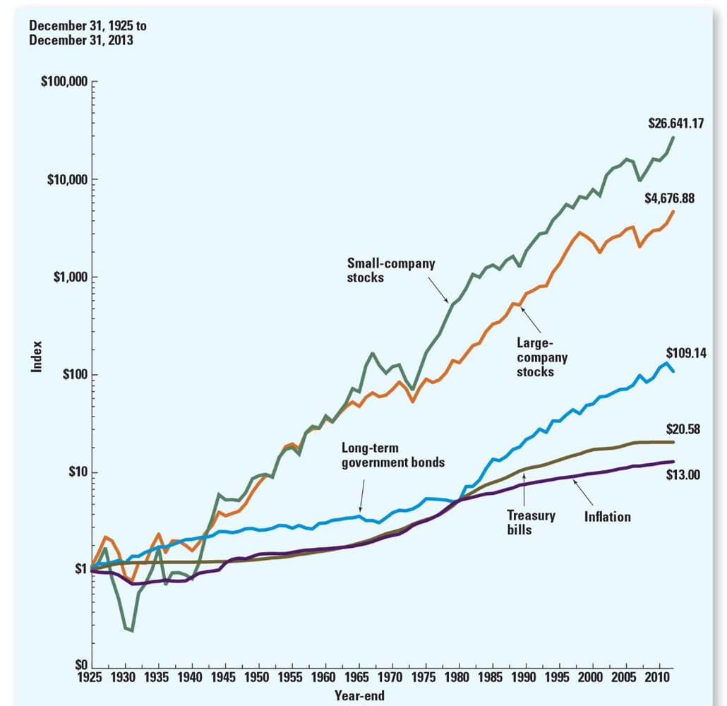
Ranking Returns
- Small cap stocks
- Large cap stocks
- Long-term government bonds
- Treasury Bills
- Inflation
Why wouldn't you just buy small cap stocks?
Calculating Returns
- Total Dollar Return
- $Return = Dividends + Capital Gains
- Total Percent Return
- %Return = $\frac{\$Return}{\$Invested}$
Example: Returns
You just invested in "You call that a Donut! Inc" for $\$$25, after one-year the price is $\$$35. Each share paid out a $\$$2 dividend. What was your total return?| Dollar Return | Percent Return | |
|---|---|---|
| Dividend | 2 | $\frac{2}{25}=8\%$ |
| Capital Gains | 35-25=10 | $\frac{35-25}{25}=40\%$ |
| Total Return | 2+10=12 | $\frac{10+2}{25}=48\%$ |
Percent Returns: Formulas
Dividend Yield$DY=\frac{D_{t+1}}{P_t}$
Capital Gains Yield
$CGY=\frac{P_{t-1}-P_t}{P_t}$
$\%Return=\frac{D_{t+1}+P_{t+1}-P_t}{P_t}$
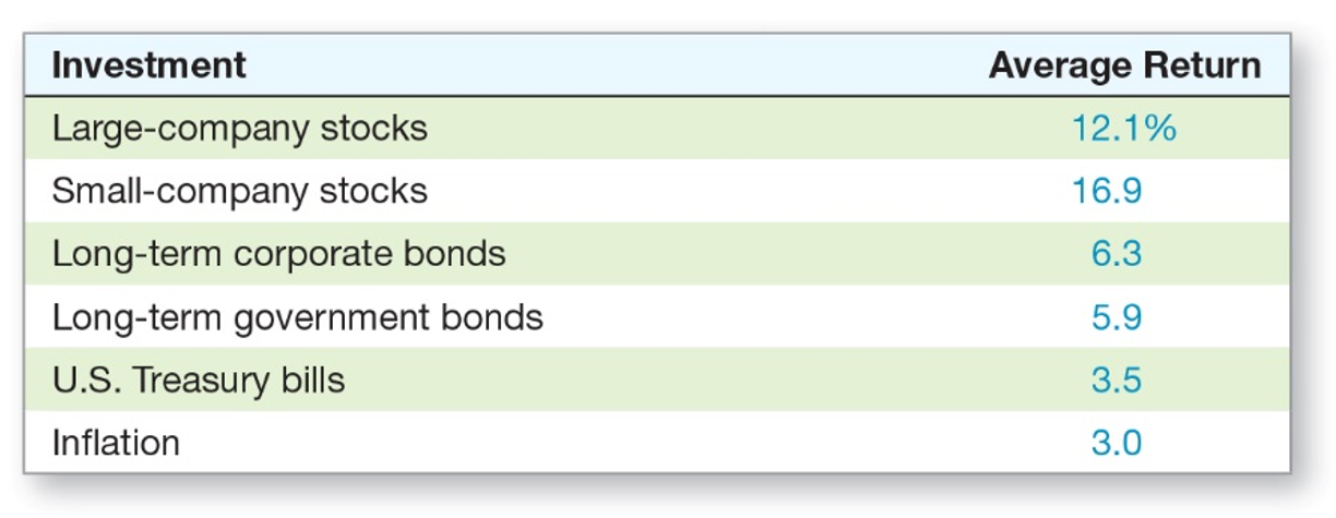
Historical Average Returns
$HistoricalAverageReturn=\frac{\sum\limits_{i=1}^TReturn_i}{T}$
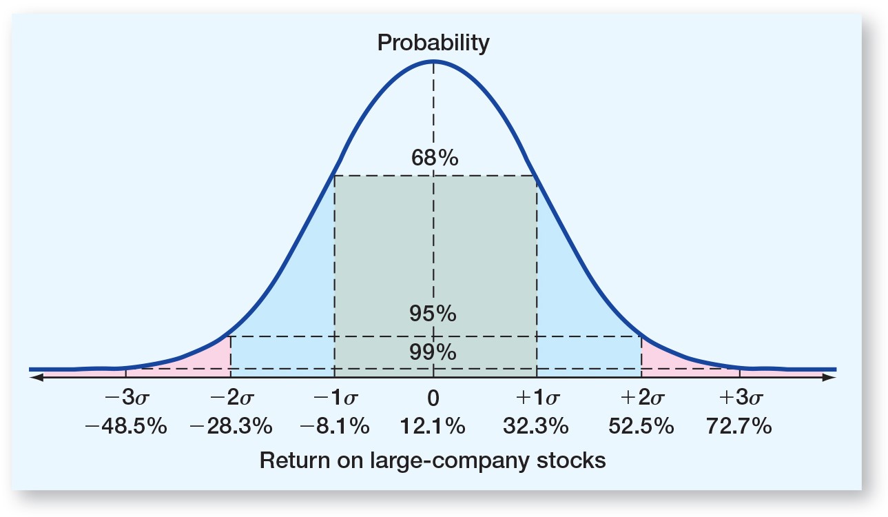
Large cap stocks average return from 1926 to 2010: 12.1%
Your best guess about the size of the return for a year selected at random is 12.1%.
Historical Average Returns: 1926-2010
Practice: Average
Returns: -6, 8, 12, -15, 6Average = 1
Returns: -1, 2, -1, 1, 4
Average = 1
Risk Premium
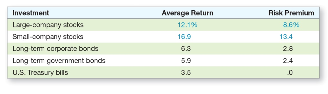
U.S. Treasury bill is considered risk-free return
Historical Average Risk Premium
First Lesson Takeaways
Large company stocks have a historical average risk premium of 8.6%
What determines size of risk premium?
Second Lesson: Return Variability
Measuring Return Variability
- Variance or $\sigma^2$
- Common measure of return dispersion
- Standard deviation or $\sigma$
- Sometimes called volatility
- Same "units" as the average
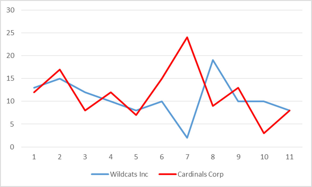
Example
Two companies have the following returns:Wildcat Inc: 13,15,12,10,8,10,2,19,10,10,8
Cardinals Corp: 12,17,8,12,7,15,24,9,13,3,8
| Wildcats Inc. | Cardinals Corp. | |
|---|---|---|
| Average | 10.6 | 11.6 |
| Standard Deviation | 4.3 | 5.7 |
Graphical Representation
Steph vs LeBron (Points in 2016 Playoffs)
Steph Curry (9 games leading into finals):40,29,26,28,24,19,31,31,36.LeBron James (9 games leading into finals):27,24,21,24,23,24,29,23,33.
| Steph | LeBron | |
|---|---|---|
| Average | 29.33 | 25.33 |
| Standard Deviation | 6.25 | 3.71 |
Return Variability
- Return Variance:
$VAR(R)=\sigma^2=\frac{\sum\limits_{i=1}^T(R_i-\bar{R})^2}{T-1}$
- Standard deviation:
$STD(R)=\sigma=\sqrt{VAR(R)}$
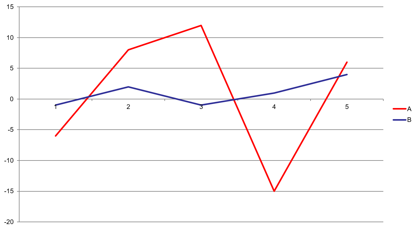
Practice: Standard Deviation
Returns(A): -6, 8, 12, -15, 6Average = 1
Standard deviation = 11.18
Returns(B): -1, 2, -1, 1, 4
Average = 1
Standard deviation = 2.12
Graphing Returns
Example
| Year | Return (%) | Average Return (%) | Difference | Squared Difference |
|---|---|---|---|---|
| 1926 | 11.14 | 11.48 | -.034 | 0.0012 |
| 1927 | 37.13 | 11.48 | 25.65 | 657.82 |
| 1928 | 43.31 | 11.48 | 31.83 | 1013.02 |
| 1929 | -8.91 | 11.48 | -20.39 | 415.83 |
| 1930 | -25.26 | 11.48 | -36.74 | 1349.97 |
| Variance | 859.19 | |||
| Standard Deviation | 29.31 |
Normal Distribution
Arithmetic vs. Geometric Mean
Think about returns...
If you invest in a hedge fund that loses 20% the first year, but makes 20% the second year, are you back to even?- NO!!!!!
- Start with $\$$100
- After year 1: you have $\$$80
- After year 2, you have $96
Another example
Suppose you invest $\$$100 and it falls 50% in year one but gain 100% in year 2.- Year 0:100
- Year 1:100*(1-0.50)=50
- Year 2:50*(1+1)=100
Arithmetic vs. Geometric Mean
- Arithmetic average:
- Return earned in an average period over multiple periods
- Answers the question: "What was your return in an average year over a particular period?"
- Geometric average
- Average compound return per period over multiple periods
- Answers the question: "What was your average compound return per year over a particular period?"
Geometric average < Arithmetic average unless all the returns are equal
Geometric Average: Formula
$GAR=[(1+R_1)*(1+R_2)*...*(1+R_T)]^{\frac{1}{T}}-1$
Where:
$R_i$= return in each period
$T$ = number of periods
Geometric Average: Formula
$GAR=[\prod\limits_{i=1}^T(1+R_i)]^{\frac{1}{T}}-1$
Where:
$\prod$= Symbol for product (multiply)
$R_i$= return in each period
$T$ = number of periods in sample
Revisit Examples
If you invest in a hedge fund that loses 20% the first year, but makes 20% the second year.Average Return: 0%
Geometric return: -2.02%
Suppose you invest $\$$100 and it falls 50% in year one but gain 100% in year 2.
Average Return: 25%
Geometric Return: 0%
Example
| Year | Return (%) | (1+R) | Compounded |
|---|---|---|---|
| 1926 | 11.14 | 1.114 | 1.114 |
| 1927 | 37.13 | 1.3713 | 1.5241 |
| 1928 | 43.31 | 1.4331 | 2.1841 |
| 1929 | -8.91 | 0.9109 | 1.9895 |
| 1930 | -25.26 | 0.7474 | 1.4870 |
| $(1.4870)^\frac{1}{5}$ | 1.0826 | ||
| Geometric return | 8.26% |
Capital Market Efficiency
Capital Market Efficiency
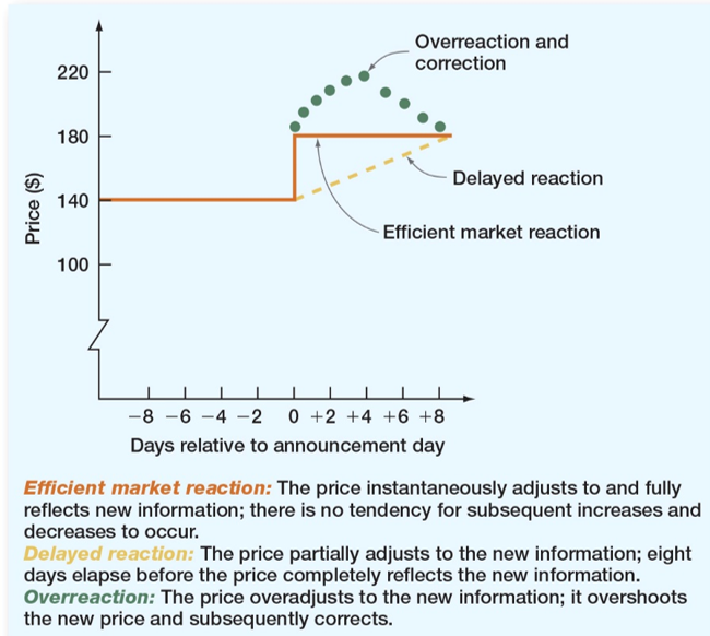
If true, cannot earn abnormal or excess returns.
Efficient Market Hypothesis
- Idea is competition among investors drives information into prices and thus the market becomes more and more efficient.
- Stocks are all priced correctly
Finance version of "Dad Joke"
A student and a finance professor are walking down the hall when they both see a $\$$20 bill on the ground. The student bends down to pick it up.The professor shakes their head slowly with a look of disappointment. And says…
"Don't bother, If it were really there, someone else would have picked it up already"
Forms of Market Efficiency
- Strong form: all information of every kind is reflected in the stock prices. Including public and private.
- Semi-strong form: all public information is reflected in stock prices.
- Weak form: Prices reflect all past trading information such as prices and volume.
Summary
- No simple way to "beat" the market
- Identifying mispriced stocks is very difficult (borderline impossible)
- Prices do respond rapidly to information
- Very difficult to predict future stock prices
Expected Returns and Variances
Weighted Average Reminder
Your grade is weighted 30% for the midterm 50% for the final. Homework is worth 10% and quizzes another 10%. You did perfect on the homework and quizzes. The midterm you received a 81 and the final was an 92. What is your final grade?Answer: 90.3
Expected Returns
- Expected returns are based on the probabilities of possible outcomes
- In this context, "expected" means average if the process is repeated many times
- The "expected" return does not even have to be a possible return
$E(R)=\sum\limits_{i=1}^Np_iR_i$
Example: E(R)
Suppose you have predicted the following returns for stocks C and T in three possible states of the economy. What are the expected returns?| State | Probability | C | T |
|---|---|---|---|
| Boom | 0.3 | 0.15 | 0.25 |
| Normal | 0.5 | 0.1 | 0.2 |
| Recession | ??? | 0.02 | 0.01 |
| Expected Return | 9.9% | 17.7% |
Variance and Standard Deviation
- Variance and standard deviation measure the volatility of returns
- Using unequal probabilities for the entire range of possibilities
- Weighted average of squared deviations
$\sigma^2=\sum\limits_{i=1}^np_i(R-E(R))^2$
Example
| State | $P_i$ | C | T | $p_i(R_C-E(R))^2$ | $p_i(R_T-E(R))^2$ |
|---|---|---|---|---|---|
| Boom | 0.3 | 0.15 | 0.25 | $0.3(0.15-0.099)^2$ | $0.3(0.25-0.177)^2$ |
| Normal | 0.5 | 0.1 | 0.2 | $0.5(0.1-0.099)^2$ | $0.5(0.2-0.177)^2$ |
| Recession | 0.2 | 0.02 | 0.01 | $0.2(0.02-0.099)^2$ | $0.2(0.01-0.177)^2$ |
| $\sigma^2$ | 0.002029 | 0.007441 | |||
| $\sigma$ | 4.50% | 8.63% |
Portfolios
What is a portfolio?
- A portfolio is a collection of assets
- An asset's risk and return are important in how they affect the risk and return of the portfolio
- The risk-return trade-off for a portfolio is measured by the portfolio expected return and standard deviation, just as with individual assets
Portfolio Weights
Suppose you have $\$$15,000 to invest and you have purchased securities in the following amounts. What are your portfolio weights in each security?| Portfolio | Weights |
|---|---|
| $\$$2000 of DIS | 2/15=13.33% |
| $\$$3000 of KO | 3/15=20% |
| $\$$4000 of AAPL | 4/15=26.7% |
| $\$$6000 of PG | 6/15=40% |
Portfolio Expected Return
$E(R_p)=\sum\limits_{j=1}^mw_jE(R_j)$
- You can also find the expected return by finding the portfolio return in each possible state and computing the expected value as we did with individual securities
Example
| Stock | Weight | Return | $w_jE(R_j)$ |
|---|---|---|---|
| DIS | .1333 | 19.69% | 2.62% |
| KO | .20 | 5.25% | 1.05% |
| AAPL | .267 | 16.65% | 4.45% |
| PG | .40 | 18.24% | 7.30% |
| $E(R_p)$ | 15.41% |
Portfolio Variance
- Compute the portfolio return for each state.
- Compute the expected portfolio return using the same formula as for an individual asset.
- Compute the portfolio variance and standard deviation using the same formulas as for an individual asset.
Example
| State | $P_i$ | A (50%) | B (50%) | $E(R_{p,i})$ | $p_i(E(R_{p,i})-E(R_p))^2$ |
|---|---|---|---|---|---|
| Boom | .4 | 30% | -5% | 12.5% | $.4(12.5-9.5)^2=3.6$ |
| Bust | .6 | -10% | 25% | 7.5% | $.6(7.5-9.5)^2=2.4$ |
| $E(R_j)$ | 6% | 13% | $E(R_p)$9.5% | $\sigma_p^2$=6 | |
| $\sigma_j^2$ | 384 | 216 | $\sigma_p$=2.45% | ||
| $\sigma_j$ | 19.6% | 14.7% |
Note: You CANNOT use stock level $\sigma^2$ and $\sigma$ to calculate portfolio.
Risk, Return, and Diversification
Systematic Risk
- Risk factors that affect a large number of assets
- Also known as non-diversifiable risk or market risk
- Includes such things as changes in GDP, inflation, interest rates, etc.
Unsystematic Risk
- Risk factors that affect a limited number of assets
- Also known as unique risk and asset-specific risk
- Includes such things as labor strikes, part shortages, etc.
Returns
$Total Return = Expected Return + Unexpected Return$$Unexpected Return = Systematic Portion $
$+ Unsystematic Portion$
$Total Return= Expected Return + Systematic Portion$
$+ Unsystematic Portion$
Diversification
- Diversification is not just holding a lot of assets
- For example, if you own 50 Internet stocks, you are not diversified
- However, if you own 50 stocks that span 20 different industries, then you are diversified
The Principle of Diversification
- Diversification can substantially reduce the variability of returns without an equivalent reduction in expected returns
- This reduction in risk arises because worse than expected returns from one asset are offset by better than expected returns from another
- However, there is a minimum level of risk that cannot be diversified away and that is the systematic portion
Diversifiable vs Non-Diversifiable Risk
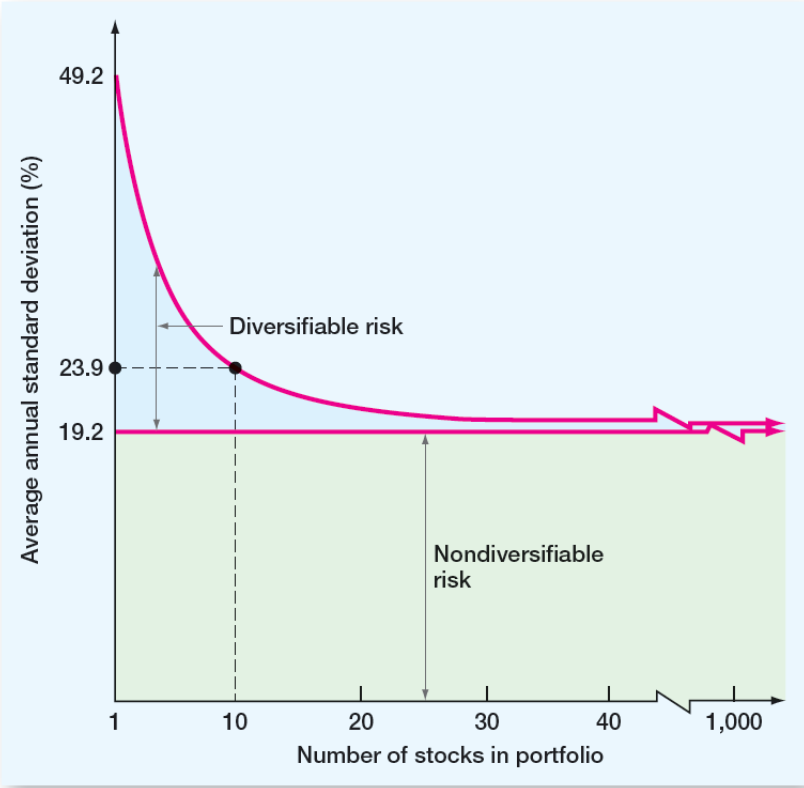
Diversifiable Risk
- The risk that can be eliminated by combining assets into a portfolio
- Often considered the same as unsystematic, unique or asset-specific risk
- If we hold only one asset, or assets in the same industry, then we are exposing ourselves to risk that we could diversify away
Total Risk
- The standard deviation of returns is a measure of total risk
- For well-diversified portfolios, unsystematic risk is very small
- Consequently, the total risk for a diversified portfolio is essentially equivalent to the systematic risk
Systematic Risk Principle
Measuring Systematic Risk
- How do we measure systematic risk?
- We use the beta coefficient
- What does beta tell us?
- A beta of 1 implies the asset has the same systematic risk as the overall market
- A beta < 1 implies the asset has less systematic risk than the overall market
- A beta > 1 implies the asset has more systematic risk than the overall market
Current Beta's
Total vs. Systematic Risk
Consider the following information:| Standard Deviation | Beta | |
|---|---|---|
| Marathon Oil | 20% | 3.13 |
| Exxon Mobil | 30% | 0.69 |
- Which security has more total risk? Exxon Mobil
- Which security has more systematic risk? Marathon Oil
- Which security should have the higher expected return? Marathon Oil
Portfolio Beta
Consider the previous example with the following four securities| Security | Weight | Beta |
|---|---|---|
| DIS | .133 | 1.444 |
| KO | .2 | 0.797 |
| AAPl | .267 | 1.472 |
| PG | .4 | 0.647 |
What is the portfolio beta?
.133(1.444) + .2(0.797) + .267(1.472) + .4(0.647) = 1.003
Portfolio Expected Returns and Betas
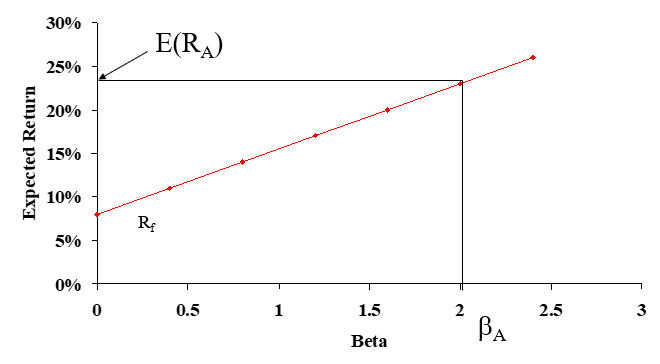
Reward-to-Risk Ratio
- The reward-to-risk ratio is the slope of the line illustrated in the previous example
- $Slope=\frac{E(R_A)-R_f}{\beta_A-0}$
- From graph, $Slope=\frac{23-8}{2-0}=7.5$
- What if an asset has a reward-to-risk ratio of 8 (implying that the asset plots above the line)?
- What if an asset has a reward-to-risk ratio of 7 (implying that the asset plots below the line)?
Market Equilibrium
$\frac{E(R_A)-R_f}{\beta_A}=\frac{E(R_M)-R_f}{\beta_M}$
Security Market Line
- The security market line (SML) is the representation of market equilibrium
- The slope of the SML is the reward-to-risk ratio: $\frac{E(R_M)-R_f}{\beta_M}$
- But since the beta for the market is always equal to one, the slope can be rewritten
- Slope $=E(R_M) – R_f =$ market risk premium
Put it all together...
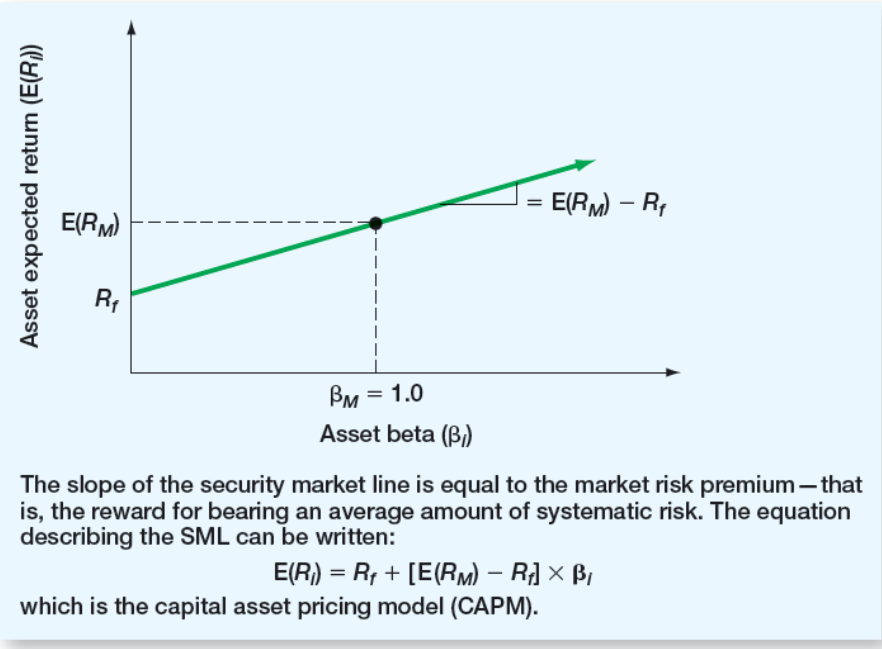
The Capital Asset Pricing Model (CAPM)
$E(R_i)=R_f+\beta_i(E(R_M)-R_f)$
- If we know an asset's systematic risk, we can use the CAPM to determine its expected return
- This is true whether we are talking about financial assets or physical assets
Factors Affecting Expected Return
- Pure time value of money: measured by the risk-free rate
- Reward for bearing systematic risk: measured by the market risk premium
- Amount of systematic risk: measured by beta
CAPM: Example
Consider the betas for each of the assets given earlier. If the risk-free rate is 4.15% and the market risk premium is 8.5%, what is the expected return for each?| Asset | Beta | $E(R_i)$ |
|---|---|---|
| DIS | 1.444 | 4.15 + 1.444(8.5) = 16.42% |
| KO | 0.797 | 4.15 + 0.797(8.5) = 10.92% |
| AAPL | 1.472 | 4.15 + 1.472(8.5) = 16.66% |
| PG | 0.647 | 4.15 + 0.647(8.5) = 9.65% |
Extra Practice
Example 1
One year ago, Avril purchased 3,600 shares of Lavigne stock for $\$$101,124. Today, she sold those shares for $\$$26.60 a share. What is the total return on this investment if the dividend yield is 1.7 percent?Example 2
A stock has yielded returns of 6 percent, 11 percent, 14 percent, and -2 percent over the past 4 years, respectively. What is the standard deviation of these returns?Example 3
You purchased 1,300 shares of LKL stock 5 years ago and have earned annual returns of 7.1 percent, 11.2 percent, 3.6 percent, -4.7 percent and 11.8 percent. What is your arithmetic average return?What is the geometric return?Example 4
What is the expected return, variance, and standard deviation?| State | Probability | Go Nuts for Donuts Inc. |
|---|---|---|
| Boom | .25 | .15 |
| Normal | .5 | .08 |
| Slowdown | .15 | .04 |
| Recession | .10 | -.03 |
Example 5
Consider the following information on returns and probabilities:| State | Probability | Apple | Disney |
|---|---|---|---|
| Boom | .25 | 15% | 10% |
| Normal | .6 | 10% | 9% |
| Recession | .15 | 5% | 10% |
What are the expected return and standard deviation for a portfolio with an investment of $\$$6,000 in Apple and $\$$4,000 in Disney?
Example 6
The risk free rate is 4%, and the required return on the market is 12%.- What is the required return on an asset with a beta of 1.5?
- What is the reward/risk ratio?
- What is the required return on a portfolio consisting of 40% of the asset above and the rest in an asset with an average amount of systematic risk?
Why Cost of Capital is Important?
- We know that the return earned on assets depends on the risk of those assets
- The return to an investor is the same as the cost to the company
- Our cost of capital provides us with an indication of how the market views the risk of our assets
- Knowing our cost of capital can also help us determine our required return for capital budgeting projects
Required Return
- The required return is the same as the appropriate discount rate and is based on the risk of the cash flows
- We need to know the required return for an investment before we can compute the NPV and make a decision about whether or not to take the investment
- We need to earn at least the required return to compensate our investors for the financing they have provided
Financial Policy and Cost of Capital
Big picture
- A firm's cost of capital reflects the required return on the firm's assets as a whole
- A firm uses both debt and equity capital
- Cost of capital will be a mixture
Cost of Equity
- The cost of equity is the return required by equity investors given the risk of the cash flows from the firm
- There are two major methods for determining the cost of equity
- Dividend Growth Model
- SML, or CAPM
DGM Approach: Reminder
$R_E=\frac{D_1}{P_0}+g$
DGM: Pros and Cons
- Advantages
- easy to understand and use
- Disadvantages
- Requires a dividend payment
- Requires growth rate to be constant
- Extremely sensitive to growth rate estimate
- Does not explicitly consider risk
SML Approach: Reminder
$R_E=R_f+\beta_E(E(R_M)-R_f)$
SML or CAPM: Pros and Cons
- Advantages
- Explicitly adjusts for systematic risk
- Applicable to all companies, as long as we can estimate beta
- Disadvantages
- Have to estimate the expected market risk premium, which does vary over time
- Have to estimate beta, which also varies over time
- We are using the past to predict the future, which is not always reliable
Cost of Debt
- The cost of debt is the required return on our company's debt
- We usually focus on the cost of long-term debt or bonds
- The required return is best estimated by computing the yield-to-maturity on the existing debt
- The cost of debt is NOT the coupon rate
Weighted Average Cost of Capital (WACC)
- We can use the individual costs of capital that we have computed to get our "average" cost of capital for the firm
- This "average" is the required return on the firm's assets, based on the market's perception of the risk of those assets
- The weights are determined by how much of each type of financing is used
Capital Structure Weights
- Notation
- E = market value of equity = # of outstanding shares times price per share
- D = market value of debt = # of outstanding bonds times bond price
- V = market value of the firm = D + E
- Weights
- $w_E = \frac{E}{V} =$ percent financed with equity
- $w_D=\frac{D}{V}=$ percent financed with debt
Taxes
- We are concerned with after-tax cash flows, so we also need to consider the effect of taxes on the various costs of capital
- Interest expense reduces our tax liability
- This reduction in taxes reduces our cost of debt
- Dividends are not tax deductible, so there is no tax impact on the cost of equity
WACC
$WACC=w_ER_E+w_DR_D(1-T_C)$
Large Example
Go Nuts for Donuts! Inc.
Go Nuts for Donuts! Inc. has 50,000,000 shares outstanding that currently trade at $\$$80 a share. The firm recently paid a dividend of $\$$3.5 and its past 5-year growth rate in dividends is 6%. It's systematic risk, measured by beta, is 1.15. The firm has $\$$1 billion in outstanding debt, face value. The current quote on the bond is 110 and the coupon rate is 9% (semi-annual coupon payments). The bonds have 15 years to maturity. Assume a tax rate of 40%. The market risk premium is 9% and the risk free rate is 5%.Solution: Cost of Equity
What is the Cost of Equity?
- Dividend Growth Model $R_E=\frac{D_1}{P_0}+g=\frac{3.5(1.06)}{80}+.06=.106375=10.64%$
- CAPM $R_E=R_f+\beta_E(E(R_M)-R_f)=5+1.15(9)=15.35%$
Solution: Cost of Debt
What is the Cost of Debt?
- N=15*2=30
- I%=3.927*2=$7.854=R_D$
- PV=-1100
- PMT=90/2=45
- FV=1000
What is the After-Tax Cost of Debt?
$R_D(1-T_C)=7.854(1-.4)=4.712%$
Solution: Weights
What are the capital structure weights?
- E=50,000,000*80= 4 billion
- D=1,000,000,000*1.1=1.1 billion
- V=4 + 1.1 = 5.1 billion
- $w_E=\frac{E}{V}=\frac{4}{5.1}=.7843$
- $w_D=\frac{D}{V}=\frac{1.1}{5.1}=.2157$
Solution
What is the WACC?
- Using DGM: $WACC=w_ER_E+w_DR_D(1-T_C)$
- Using CAPM: $WACC=w_ER_E+w_DR_D(1-T_C)$
$WACC=.7843(10.64)+.2157*(7.854(1-.4)=9.36$
$WACC=.7843(15.35)+.2157*(7.854(1-.4)=13.06$
Issues with WACC
SML and WACC
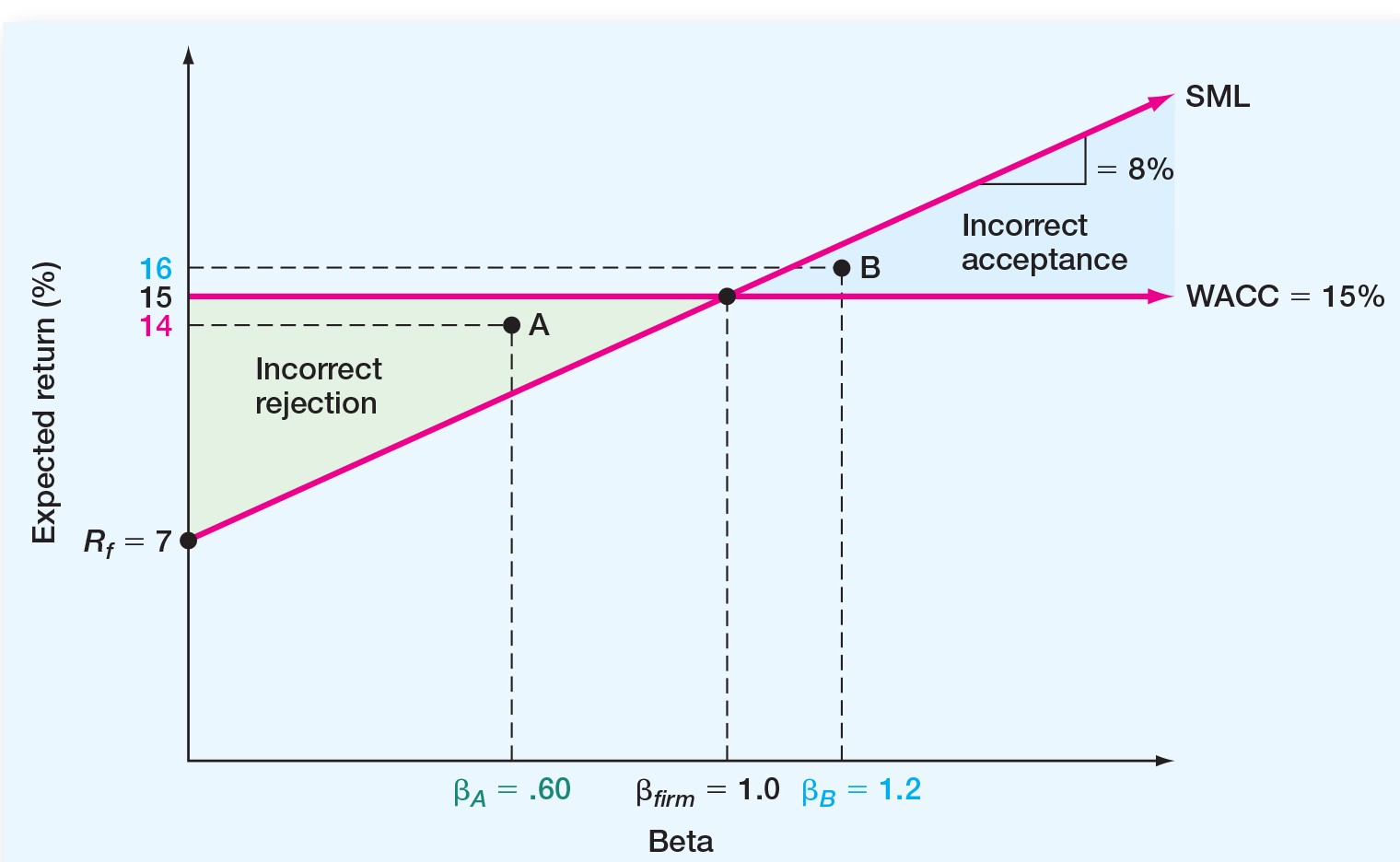
Divisions and WACC
- Using firm-level WACC can lead to:
- Incorrectly accepting high risk projects if $\beta$ of project is higher
- Incorrectly rejecting low risk projects if $\beta$ of project is lower
- Solutions:
- Pure Play: Use similar investment(company) in marketplace
- Subjective: Make risk adjustments to WACC.
Extra Practice
Example 1
- Suppose your company has an equity beta of .58, and the current risk-free rate is 6.1%. If the expected market risk premium is 8.6%, what is your cost of equity capital?
- Suppose that your company is expected to pay a dividend of $\$$1.50 per share next year. There has been a steady growth in dividends of 5.1% per year and the market expects that to continue. The current price is $\$$25. What is the cost of equity?
- Suppose we have a bond issue currently outstanding that has 25 years left to maturity. The coupon rate is 9%, and coupons are paid semiannually. The bond is currently selling for $\$$908.72 per $\$$1,000 bond. What is the cost of debt?
Example 2
Suppose you have a market value of equity equal to $\$$500 million and a market value of debt equal to $475 million. What are the capital structure weights?Example 3
A corporation has 10,000 bonds outstanding with a 6% annual coupon rate, 8 years to maturity, a $\$$1,000 face value, and a $\$$1,100 market price. The company's 500,000 shares of common stock sell for $\$$25 per share and have a beta of 1.5. The risk free rate is 4%, and the market return is 12%. Assuming a 40% tax rate, what is the company’s WACC?Key Learning Outcomes
- First Lesson: Average Returns
- Historical returns
- Risk Premium
- Second Lesson: Return Variability
- Standard deviation
- Arithmetic vs Geometric return
- Capital market efficiency
- Efficient market hypothesis
Key Learning Outcomes
- Calculate:
- Expected return, variance, and standard deviation
- Do so for a portfolio of assets
- Understand diversification
- Total risk, Systematic risk, Unsystematic risk
- Beta, Security Market Line and CAPM
- Understand concept and derivation
- Calculate Portfolio Beta
- Use CAPM
Notes on Notations
$R$= Return$R_i$= Return for stock i (index (i) can be i, j, or any letter)
$\sigma^2_i$ Variance for stock i
$\sigma_i$ Standard deviation for stock i
$E(R_i)$= Expected return for stock i
$E(R_p)$= Expected return for a portfolio
$p_i$= Probability of state i occurring
$E(R_{p,i})$= Expected return of the portfolio in state i
$R_f$= risk free rate or expected return on the risk free asset
$\beta_i$= Beta of stock i $\beta_m$= Beta of the market (equal to one)